WISE Bootstrapping Applet: Demonstration Guide
This guide can be viewed as a webpage or downloaded:
Bootstrap Guide
Purpose of the Bootstrapping Applet
The WISE Bootstrapping Applet allows instructors to illustrate
the underlying process of creating bootstrapped confidence intervals. It
demonstrates how population shape and variance, sample size, and number of
resamples affect bootstrapped confidence intervals for mean and medians. The
applet can be found at Bootstrapping Applet.
Brief Explanation of Logic
Bootstrapping is based on the premise that a random sample from a population
provides the best available information about the distribution of that population,
rather than the conventional automatic assumption that the population distribution is
normal. Bootstrapping involves drawing many random samples, with replacement, from the
original sample to generate the distribution of possible sample statistics one could
have obtained from a population shaped like the original sample.
Instructors can use the WISE Bootstrap Applet to show each step of the bootstrapping process
in detail. The applet shows the underlying population, the original sample, each resample,
and the distribution of resampled means or medians, with 95% confidence intervals for the population
parameter.
At the end of this document is a chart that can be used as a quick reference for the components
of the applet. During a demonstration of an applet, it is vital that students understand what the
various components represent, the purpose and the interpretation for each step, as well as an
interpretation of the final results.
Teaching Examples
- Setup: Display the WISE Bootstrapping Applet
 |
a. You may wish to increase the size of the display. |
| b. Slide the orange n bar to n = 16 |
| c. Set Reps = 1 |
| d. Set Statistic to: Mean |
- Confidence Interval for the Population Mean: normal distribution n = 16
 |
a. Begin with a scenario that will be of interest to the students. For example:
“We would like to estimate the average battery life for a new electronic device:
noise-cancelling headphones. The average from a random sample of headphones can be used to provide this estimate, but
we recognize that there is sampling error. Thus, along with the estimate of the average,
it is useful to have confidence limits that specify likely bounds for the true population
average. The traditional approach to constructing confidence intervals is to assume the
sampling distribution of means to be normal. Often, this assumption can be questioned.
Bootstrapping provides confidence intervals with no assumptions regarding the shape of
the population distribution. For illustration, we will begin with a normal population
distribution, but then apply bootstrapping to a non-normal distribution.”
|
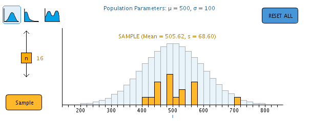
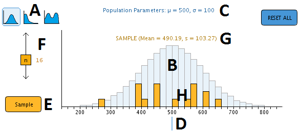
| b. Describe the blue population distribution on the display. This represents the true distribution of battery life of the headphones. The mean and standard deviation are shown as 500 and 100, respectively. We never actually see the true population distribution. All we will have is one sample of headphones which we will use to draw inferences about the population distribution. Suppose we collect data on the battery life from a random sample of 16 headphones. We can simulate this by pressing the orange Sample button.
|
| c. Click “Sample.” Note that the orange boxes indicate the 16 sampled cases. We can count the number of observations in each bin. The sample mean and standard deviation are shown in orange above the distribution. The blue line represents the population mean, a value that we don’t know but we would like to estimate.
|
| d. In practice, we never see the true population distribution. All we have is the observed sample distribution. Using this orange original sample as our best estimate of the population distribution, we can draw samples from it to represent other possible samples that we might have obtained from a population that looks like our original sample.
|
| 
|
|
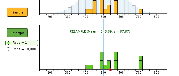
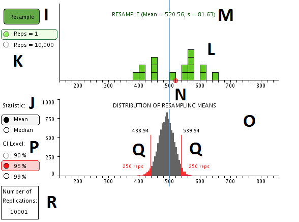
e. Click “Resample” to simulate drawing a sample from our original sample distribution. A key point here is to show that the green resample is drawn with replacement from the original sample. That is, some values may be drawn more than once and some may not be drawn at all. Point out examples. The mean and standard deviation for the resample are shown in green above the resampled distribution. A red mark shows the mean of this resampled distribution. This mean is also shown in the bottom graph as one possible mean for a sample of n = 16 drawn from a population that looks like our original sample.
|
| 
|
|
f. Click “Resample” again to simulate another sample that could have come from a population that looks like our original sample. Describe how this resampled distribution differs from the first resampled distribution, though both represent possible distributions from a population that looks like the original orange sample.
|
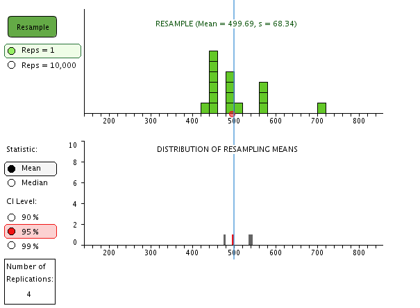
| g. Click “Resample” several more times and observe how the means of the resampled distributions vary, as recorded in the bottom graph. The bottom graph gives information about the variability of sample means for samples of size n = 16 drawn from a population that looks like the original orange sample.
|
|  |
|
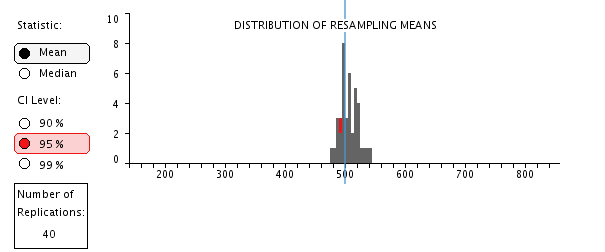
h. Check to make sure students understand the resampling process and the distribution of resampled means. Click “Resample” many more times to bring the total number of resampled means to 40. The distribution of resampling means is beginning to take shape, and it gives a rough sense of the range of possible sample means. However, with only 40 resampled means, the distribution is still quite unstable. A more stable distribution can be generated by using the computer to generate a very large number of replications.
|
| 
|
|
i. Under the green Resample button, select Reps = 10,000. Click Resample.
|
| 
|
|
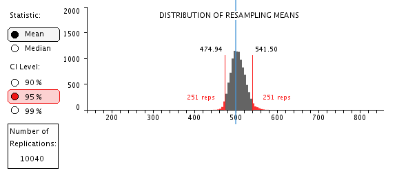
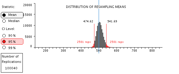
j. The distribution of resampling means now shows the distribution for 10040 resampled means. A 95% confidence interval for such means can be determined by finding the limits that cut off the upper 2.5% and the lower 2.5% of the distribution. With 10040 cases, the 2.5% tails include 251 cases each. The applet shows these limits to two decimal places. That may be more precise than is warranted. We can easily increase the number of resampled means by clicking the Resample button repeatedly. Generally, the distribution will become smoother, but little is gained by increasing the number of resamples. The figure belolw shows 100,040 resampled means.
|
| 
|
Interpretation:
Based on the random sample of 16 headphones, we have 95% confidence that the actual average battery life of this brand of headphones is between 474 and 542 minutes.
Compare to parametric confidence interval (optional):
In this example, the population distribution was normal, so the sampling distribution of the means is normal, and conventional computations for a confidence interval would be appropriate. In the example here, the standard deviation from the original sample is 68.60 so with the sample size of n = 16, the estimated standard error of the mean is 68.60/4 = 17.15. With df = 15, t = 2.13 for a two-tailed test with alpha of .05. This gives error around the sample mean (505.62) of 17.15 * 2.13 = 36.53, so the parametric confidence bounds are 505.62 – 36.53 = 469.09 and 505.62 + 36.53 = 542.15. This compares to the resampling bounds of 474.62 and 541.69.
- Confidence Interval for the Population Mean: skewed distribution, n = 16
|
a. Check settings: n = 16; Reps = 10,000; Statistic: Mean
|
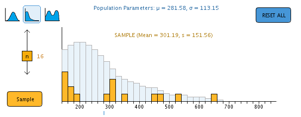
| b. Change the shape of the population to a highly skewed distribution. You can use the pre-set skewed distribution by clicking the blue skewed population icon at the top left of the applet. If you want to create your own skewed distribution, you can hold the left mouse button down as you move your mouse to draw the desired shape, or you can click on the desired height for any bar.
|
| c.
Click Sample to draw a sample of 16 cases from this skewed population. For the best illustration, the orange sample should reflect the strong skew as shown here.
|
|  |
|
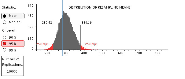
d. Click Resample with Reps = 10,000 to generate the empirical sampling distribution.
|
|  |
|
e. Note that the sampling distribution is not symmetrical, and so the confidence interval limits also are not symmetrical. In the example here, the upper limit of 380.19 is 79 above the sample mean of 301.19, while the lower limit is only (301.19 – 230.62 = 70.57 below the sample mean. These asymmetrical limits reflect the skewed population more accurately than the symmetric limits that would be obtained with the parametric procedures that assume that the sampling distribution is normal.
|
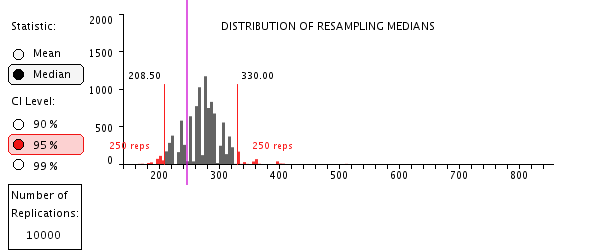
- Confidence Interval for the Population Median: skewed distribution, n = 16
|
a. When a distribution is very skewed, the median may be more descriptive and more useful than the mean. Although the parametric approach does not apply to medians, the bootstrapping method works just fine.
|
|
b. Keep settings: n = 16; Reps = 10,000; but change Statistic: Median
|
| c. You can continue to use the distribution from the previous section. Click Resample to construct the sampling distribution of the medians with 10,000 replications.
|
| d. (If you wish to use a new population distribution, set the shape of the population to a highly skewed distribution. You can hold the left mouse button down as you draw the desired shape, or you can click on the desired height for any bar. Click Sample to draw a sample of 16 cases from this skewed population. For the best illustration, the sample should reflect the strong skew.)
|
|  |
|
e. The sampling distribution of the medians is likely to be quite choppy, especially with small samples such as n = 16. Some values are impossible for medians because no cases in the sample have those values. Nonetheless, the bootstrapped sampling distribution shows the limits for the confidence interval for the population median.
|
|
f. Further discussion: From the same population, try different samples. On average, we expect 95% of the confidence intervals to capture the true population value, so about one in twenty is expected to miss. Experiment with different shapes of population distributions and different sample sizes.
|
| A |
Population Shapes |
| B |
Population |
| C |
Population Parameters |
| D |
Population Mean Bar |
| E |
Sample Button |
| F |
Sample Size Slider |
| G |
Sample Statistics |
| H |
Sample |
| I |
Resample Button |
| J |
Statistic of Interest |
| K |
(Reps) Number of Resamples |
| L |
Resample |
| M |
Resample Statistics |
| N |
Resample Mean |
| O |
Statistic of Interest Graph |
| P |
Confidence Levels |
| Q |
Confidence Limits |
| R |
Total Number of Replications |
|
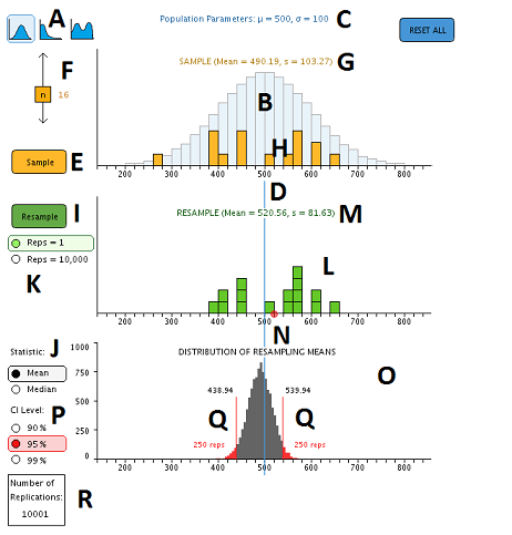 |
Pre-set population shapes are shown by the small icons on the top left of the applet (A). Clicking any icon will set the population to that shape. The population is displayed as a histogram with blue bars (B). The population shape can be altered by clicking and dragging the cursor across the graph. Clicking just below the x-axis on the graph will set the bin above the cursor to 0. Population parameters are displayed above the graph (C), and the location of the population mean is shown as a blue line that runs below the graph (D).
In order to resample, an initial sample must first be drawn. The size of the next sample can be adjusted between n = 4 and n = 39 by sliding the yellow sample size slider (F) up or down before drawing a sample.
Samples can be drawn by clicking on the Sample button (E). Sample statistics (mean and s) are displayed in orange text above the sample (G). Samples are displayed as orange bars (H) on top of the blue population graph.
After a sample is drawn, the
Resample button (I) becomes active. Either the
means or medians of future resamples can be recorded by selecting the corresponding statistic of interest
(J).
To illustrate the resampling process clearly, a single
resample can be drawn by selecting Reps = 1 with the green radio buttons
(K). With Reps = 1, one resample is taken from the initial
sample, and two important events are shown:
- The distribution of the single resample is shown in the resample graph
(L) in green, along with the resample statistics
(M).
- The mean (or
median) of the resample is displayed as a red block, and drops down from a red circle
(N) in the
resample graph into the Distribution of Resampling Means (or Medians)
(O).
The number of resamples can also be set to 10,000 by selecting the corresponding reps radio button (K). This tells the applet to resample 10,000 times on a single click of the resample button. The green distributions of these resamples are not displayed. Instead, the resulting distribution of means or medians is displayed in the bottom graph in gray (O). Further resampling simply adds upon the previous distribution of means or medians, allowing you to increase the overall number of replications indefinitely.
Confidence level can be set by selecting the desired option from the red radio buttons (P). Confidence limits are drawn in red
(Q) on the bottom graph whenever there are at least 10,000 resampled cases. These confidence limits are created at the upper and lower 2.5% of cases, resulting in a 95% confidence interval estimating either the mean or median of the population. The total number of resampling replications can be viewed at the bottom left
(R).
Last revised: January 27, 2013
|